Network analysis in GIS models how movement happens along connected infrastructure. It replaces guesswork with evidence on travel time, coverage and access, so teams can plan services, run operations and test change with confidence. This article outlines the core methods (routing, service areas and origin–destination), where they are used day to day, and the data and modelling choices that turn a map into a decision-grade network.
Network analysis scope and value
Network analysis is the part of GIS that deals with movement and connectivity: how people, vehicles, goods, water, power or information travel through connected infrastructure. In practice, it turns a map into a working model of the real world, where junctions, restrictions and capacity determine what is possible, not just what is nearby.
For public-sector teams and infrastructure operators, the value is usually operational. Network analysis helps you evidence response times, understand access and coverage, and test changes before committing budget. Done well, it replaces assumptions (“it’s about 10 minutes away”) with defensible measures (“90th percentile blue-light drive time is 11:20 at weekday peak”).
It also tends to expose data and process gaps early. For example, you might discover that the question is not “Which depot is closest?”, but “Which depot can reach the site reliably given gates, weight limits, shift patterns and turn restrictions?” Those details can be modelled, but they need to be agreed up front.
Network model basics
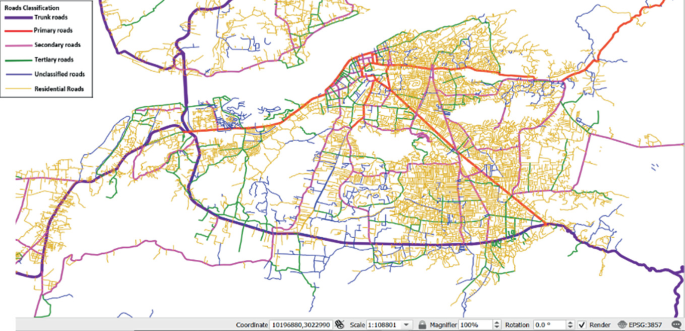
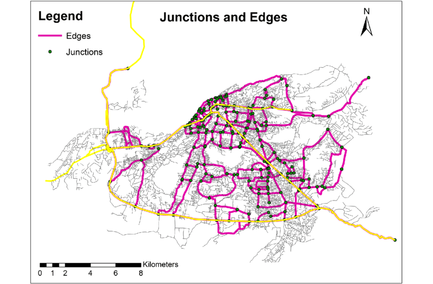
A GIS network is typically represented as edges (road segments, pipes, tracks) and junctions (intersections, valves, stops). Each edge carries costs such as distance, time, energy or risk. Connectivity rules define what can connect to what, and in which direction, critical for one-way streets, access-only roads, rail lines or pressure zones in utilities.
The practical difference between a basic network and a decision-grade network is attribution. If your road data has geometry but no turn restrictions or realistic speeds, the model will still run, but it will produce results that feel roughly right rather than operationally reliable.
Decisions supported and typical outputs
Most network analysis supports decisions about time, coverage and allocation. Common outputs include best route lines, turn-by-turn directions, isochrones (travel-time polygons) and accessibility matrices showing travel times between many origins and destinations.
On projects, these outputs often become evidence: a map for a committee report, a table for an options appraisal or a dashboard for operations. If you are new to the broader context, it helps to place this alongside other forms of spatial analysis. Network methods are distinctive because they model movement along connected infrastructure rather than straight-line proximity.
Everyday and public-sector examples
Most people interact with network analysis daily through satnav and journey planners. The same principles underpin more formal work: assessing ambulance coverage, planning gritting routes, scheduling inspections and estimating who can realistically access a service within a set time.
Local authorities also use network outputs to support policy, such as school accessibility by walking time rather than distance, or evaluating whether a proposed road closure shifts traffic onto unsuitable residential streets. The map is often the least important part; the real value is the defensible measure behind it.
Core network analysis methods
Most network projects boil down to three method families: routing (getting from A to B), service areas (what can be reached from a point) and origin–destination (how accessible opportunities are across an area). They share the same dependencies: a fit-for-purpose network, sensible assumptions and agreement on what cost means in your context.
A common misunderstanding is expecting one model to answer everything. A network built for HGV routing (weight limits, height restrictions, depot access) will not automatically be valid for walking catchments. Similarly, a public transport model needs timetables and transfer logic, not just line geometry.
Routing and vehicle paths
Routing identifies the least-cost path between locations, using distance or travel time (and sometimes penalties such as tolls, ULEZ charges or steep gradients). In the real world, the challenge is less about the algorithm and more about rules: turn restrictions, one-way streets, private access, vehicle dimensions and whether you allow U-turns.
If the output will be used operationally, by drivers, crews or dispatchers, tighten the assumptions. Agree whether you are modelling blue-light response, normal traffic compliance or HGV-compliant routing, because each needs different speeds and restrictions.
Service areas and catchments
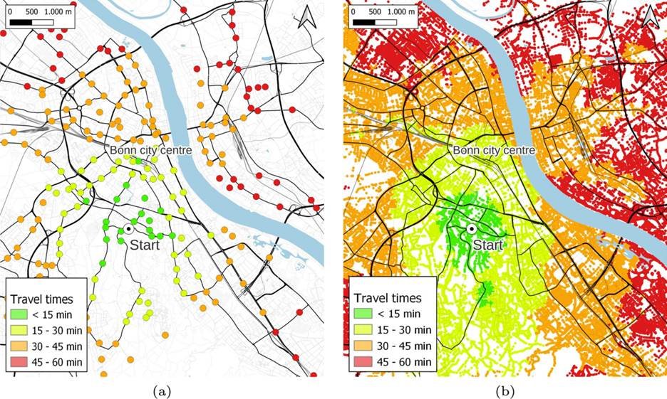
Service areas (often called isochrones) show where you can reach from a starting point within a time or distance threshold, such as “8-minute drive time from a fire station” or “15-minute walk to a GP surgery”. They are widely used for coverage analysis, standards reporting and equity assessments.
The nuance is that service areas reflect network constraints. A river with limited bridges, a motorway barrier or restricted access roads can make nearby places effectively far away. This is why service areas often replace simple circles when the question is about real access.
You can explore isochrone concepts in more depth via this guide to isochrone maps.
Origin–destination and accessibility metrics
Origin–destination (OD) analysis measures travel time or distance between many origins and many destinations. It is used for accessibility studies (for example, how many jobs are reachable within 45 minutes), catchment competition (which facility is closest by time) and scenario testing (how a new link changes connectivity).
OD outputs often look like matrices and summary indicators rather than maps. That is useful for business cases and KPIs, but it also raises performance and data issues: large OD problems can be computationally heavy, and they are very sensitive to how you represent speeds, congestion and transfers.
Planning and operations use cases
In UK projects, network analysis often sits in the middle of a workflow: you start with an operational question, translate it into a measurable network problem and deliver outputs that fit decision-making. The best projects are explicit about what will be used for planning (strategic, averaged assumptions) versus what will be used for operations (day to day, closer to real time).
It is also where stakeholders’ definitions need aligning. Response time might mean wheels rolling, arrival on scene or arrival plus setup time. Coverage might mean any reachability, or reachability with spare capacity and the right skillset. These choices materially change what the model needs to include.
Emergency response and field force dispatch
Emergency response analysis typically combines routing, service areas and OD metrics to estimate who can reach incidents within target times. For blue-light services, the assumptions are particularly important: average speeds, compliance with restrictions, station turnout time and whether you are evaluating typical conditions or worst case.
For field force dispatch (utilities, highways, housing repairs), the emphasis is often on workload balancing and travel-time reduction. Integrating live or historical job data can improve realism, but it also introduces privacy and data quality considerations, especially where address matching and timestamp accuracy are inconsistent.
Location–allocation for facilities and chargers
Location–allocation models help decide where facilities should be placed to best serve demand. That could be siting a new depot, a clinic, a recycling centre or EV chargers. The best solution depends on your objective: minimise average travel time, maximise population covered within a threshold or prioritise underserved areas.
A practical point: the model is only as good as the demand representation. Using population centroids might be acceptable for strategic work, but for local decisions you often need more granular demand points, realistic access (entrances, not just polygons) and constraints such as land availability, power capacity and planning policy.
Fleet routing and last-mile logistics
Fleet routing goes beyond shortest path to sequencing multiple stops with constraints: time windows, vehicle capacities, driver hours, depot start or end and service times at each stop. In councils, this comes up in refuse collection and highways inspections; in the private sector, it is last-mile delivery and service engineering.
Expectations need managing. You rarely get a perfect optimal plan that also fits local knowledge and operational realities. The best outcomes come from treating the model as a decision aid, then iterating with supervisors and drivers to include constraints like access gates, school streets or difficult turning locations.
If logistics is a core part of your operation, it is worth reading how GIS supports routing and logistics planning.
Multi-network applications beyond roads
Roads are the most familiar network, but the same analysis logic applies to any connected system. In consultancy work, multi-network projects often deliver the biggest value because they connect silos: transport access to service locations, utility asset connectivity to customer impact or active travel networks to planning outcomes.
They also raise more modelling questions. A pipe network has directionality, pressure zones and isolation points. Public transport has schedules and transfers. Walking networks must account for crossings, gradients and barriers. The key is being clear about what is being modelled: physical connectivity, operational rules or user experience.
1. Utility network tracing and isolation
Utility network tracing identifies how an asset is connected, such as upstream and downstream connectivity, which customers are fed by which mains, or which valves need to close to isolate a leak. For water and wastewater, this is foundational for incident response and planned works because it turns asset maps into an operational model.
The delivery risk is usually data integrity: correct connectivity, correct status (open or closed) and correct attribution (diameters, material, pressure zones). If those are wrong, the trace can be misleading. Many organisations prioritise a good-enough-for-triage trace first, then improve accuracy through targeted validation and updates.
2. Public transport accessibility and transfers
Public transport accessibility is not just distance to a bus stop. It depends on timetable frequency, wait time assumptions, interchange penalties and whether transfers are realistic for the user group. In cities, a high-frequency network may behave almost like a continuous service; in rural areas, a missed connection can add an hour.
For planners, these models are often used to evidence accessibility to jobs, education or healthcare, particularly for groups who do not drive. The trick is agreeing a sensible time-of-day and day-of-week scenario, and being explicit about whether you are reporting best case or typical conditions.
3. Walking and cycling networks in planning
Active travel analysis is usually about permeability: where people can realistically walk or cycle, given crossings, barriers, gradients and route quality. A simple road-centreline network often fails here because it misses cut-throughs, paths through parks, stairs and signed cycle routes.
For cycling, small details matter, including traffic stress, junction complexity and whether a route is suitable for different confidence levels. For walking, step-free access and crossing delay can dominate travel time. In UK planning work, these analyses often support Local Plan evidence, active travel schemes and equality-focused access assessments.
Data, modelling choices, and delivery risk
Network analysis can look deceptively simple because software makes it easy to generate routes and catchments. In delivery, most of the effort is in building a network that matches your decision context and can stand up to scrutiny.
Risk comes from three places: data fitness (are the attributes correct and current?), modelling choices (are the assumptions defensible?) and communication (are outputs interpreted appropriately?). A good brief reduces these risks by stating the intended use, accuracy needs and how results will be validated.
UK data sources and fitness for purpose
In the UK, road network data commonly comes from Ordnance Survey products, OpenStreetMap, local authority street gazetteers and transport models. Each has strengths: OS tends to be consistent and well maintained; OSM can be excellent in some areas for paths and restrictions but varies; local datasets often capture operational details like barriers and estate roads.
Fitness for purpose is about matching the dataset to the question. If you are modelling emergency response, you may need turn restrictions and realistic speeds. If you are modelling walking catchments, you need footpaths, crossings and access through open spaces. The best dataset is the one that captures the constraints that actually govern movement.
Network build requirements and constraints
Building a reliable network typically involves cleaning geometry, ensuring proper connectivity at junctions, setting direction and turn rules, and creating cost fields (time, distance or other measures). Constraints are where projects succeed or fail: vehicle restrictions, access permissions, time windows and mode-specific rules.
A common practical step is adding connectors from points like building entrances to the network. If you snap everything to the nearest road centreline without thinking, you can create unrealistic access, especially for campuses, hospitals, ports or industrial sites where entrances are controlled.
Validation, uncertainty, and scoping briefs
Validation should be proportional to how the results will be used. For strategic planning, you might sense-check a sample of routes against known journeys and confirm that catchments behave sensibly around barriers. For operational use, you may need more formal checks, comparisons against GPS tracks or stakeholder review workshops.
Uncertainty is unavoidable, so it should be communicated. Instead of implying false precision, many teams report ranges or percentiles (typical versus worst case) and document key assumptions. A strong scoping brief usually covers:
- intended decisions and users of outputs
- mode and scenario (time of day, day of week, disruption assumptions)
- constraints and business rules to encode
- deliverables (maps, tables, APIs, dashboards) and how they will be validated
That level of clarity reduces rework and makes it easier to defend results later.
Conclusion
Network analysis in GIS turns static maps into practical decision tools by modelling how movement really happens across connected systems. Whether routing vehicles, defining service coverage or measuring accessibility, its value lies in combining good data with clear assumptions to produce results that can be trusted and acted on. When scoped carefully and validated appropriately, network analysis supports better planning, more efficient operations and more transparent, evidence-based decisions.